Shifting

Using the Fourier shift property one can implement shifting of arrays not only over pixel but also sub-pixel amount.

Examples

For full interactivity, have a look at this Pluto notebook.

begin
    f(x) = cos(4π * x / 30)
    x1 = 1:30
    x2 = x1 .+ 3
end

begin
    y1 = f.(x1)
    y2 = f.(x2)
    offset = 2.01
    y3 = shift(y2, tuple(offset))
end

begin
    plot(y1, label="Original signal")
    plot!(y2, label="Shifted signal")
    plot!(y3, label="Fourier shifted with $offset")
end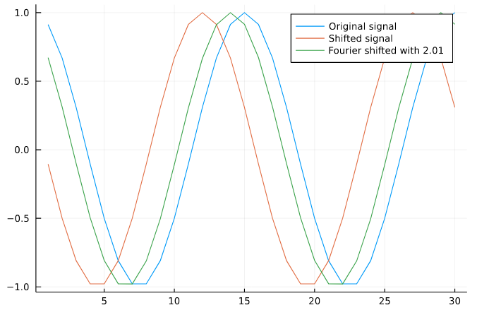

Function references

FourierTools.shift — Function

shift(arr, shifts)

Returning a shifted array. See shift! for more details

source

FourierTools.shift! — Function

shift!(arr, shifts; kwargs...)

Shifts an array in-place. For real arrays it is based on rfft. For complex arrays based on fft. shifts can be non-integer, for integer shifts one should prefer circshift or ShiftedArrays.circshift because a FFT-based methods introduces numerical errors.

kwargs...

fix_nyquist_frequency=false: Fourier shifting of even-sized arrays is not revertible. However, if you did shift(x, δ) you can it revert by shift(x, δ, fix_nyquist_frequency=true). This only works if δ is the same.
take_real=true: For even-sized arrays we take by default the real part of the exponential phase at the Nyquist frequency. This satisfies the property of real valuedness and the aliasing of the Nyquist term.

Memory Usage

Note that for complex arrays we can avoid any large memory allocations because of fft!. For rfft there does not exist a usable implementation yet, so for real arrays there might be a temporary larger memory usage.

Examples

julia> x = [1.0 2.0 3.0; 4.0 5.0 6.0]
2×3 Matrix{Float64}:
 1.0  2.0  3.0
 4.0  5.0  6.0

julia> shift!(x, (1, 2))
2×3 Matrix{Float64}:
 5.0  6.0  4.0
 2.0  3.0  1.0

julia> x = [0, 1.0, 0.0, 1.0]
4-element Vector{Float64}:
 0.0
 1.0
 0.0
 1.0

julia> shift!(x, 0.5)
4-element Vector{Float64}:
 0.49999999999999994
 0.5
 0.49999999999999994
 0.5

source